A parameter is a configurable value that changes how a detector fits data or assigns outlier scores. Choosing a detector is therefore only part of the decision: its settings can change which records appear unusual. Some detectors require no parameters; others require several, or are particularly sensitive to their values. section 3.3.7 section 3.3
Common settings affect different parts of detection:
- The number of neighbors, k, determines which points KNN and several local detectors compare. A very small k can make results variable; a very large k can bring unrelated regions into the comparison. section 8.1
- In a one-class SVM, nu influences how many training points may fall outside the fitted decision boundary. Changing the boundary trades false positives against false negatives. section 5.4
- Other settings include KDE bandwidth, DBSCAN eps, and HBOS bin count. Their appropriate values may be difficult to judge without experimentation. section 8.2.1
To examine a setting, hold the data constant and vary its value. On controlled synthetic data, compare which known global outliers, small clusters, and ordinary cluster edges receive high scores. Interpret the result against the kinds of groups the application should consider unusual: a useful k may be guided by the largest group considered an outlier and the smallest group considered normal. This is a heuristic, not a guaranteed optimum. section 8.1 section 8.1.1
Changing the neighborhood
With KNN, comparing k values of 3, 10, and 300 makes the effect visible. At k = 3, a five-point cluster can appear normal because its points have close neighbors. At k = 300, even a 50-point cluster can receive elevated outlier scores. Contours help explain the detector’s behavior in two dimensions, but they usually cannot tune a model for higher-dimensional data. section 8.2.1 section 8.8
Figure 8.5 Contour plot of the decision boundary of a KNN model using k = 3, 10, and 300. We can see the regions around the small cluster in the bottom-right are considered normal when k = 3 (as each point has this many close neighbors) but not when k is higher. When k is very high, such as 300, even fairly large clusters may receive moderate outlier scores.
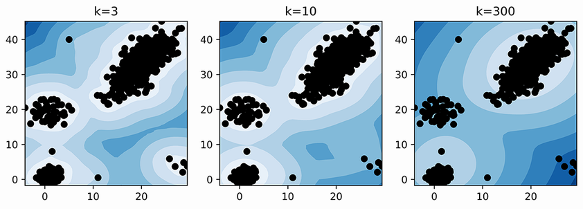
Compare the regions scored as normal or unusual under three KNN neighbor counts; the changing treatment of small and larger clusters makes the parameter’s effect concrete. section 8.2.1
When several values are plausible, fit the detector with multiple settings and combine its scores rather than relying on one choice. Combining different detectors may first require scaling their scores. Check whether the resulting high-scoring records match the intended notion of an outlier, and test fit and prediction times if the detector must handle larger workloads. A flagged record remains a candidate for examination, not an automatically meaningful anomaly. section 8.1.1 section 8.8