Backpropagation computes loss gradients in reverse through a neural network. An input gradient carries the computation to the preceding layer; a weight gradient tells the optimizer how to adjust that layer’s parameters to reduce the loss. section 5.6.1 section 6.4.1
For a linear operation written with row-oriented tensors as z = xW, let g = dL/dz be the incoming gradient. The chain rule gives dL/dx = gWᵀ and dL/dW = xᵀg. The first result continues the backward pass; the second supports the weight update. section 5.6.1
A mixed-precision backward pass
For the input-gradient calculation, an incoming BF16 gradient and the weights are converted to FP8 for multiplication. The result is accumulated in FP32, then stored in BF16 for the preceding layer. This keeps the heavy multiplication in a low-precision format while retaining more precision in the result passed between layers. section 5.6.1
Figure 5.22 The mixed-precision framework with FP8 data format in the Linear operator. The diagram illustrates the flow of data through a linear layer, showing how inputs and weights are converted to low-precision FP8 for fast computation, while critical components like master weights and gradients are maintained in high-precision FP32 for stability.
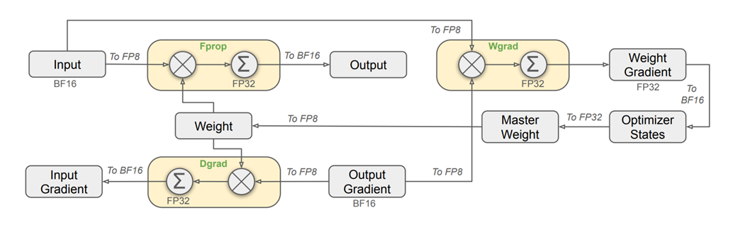
Follow the forward and backward data flows through a linear operator, including the precision formats used for weights and gradients. section 5.6.1
In a PyTorch training step, loss.backward() calculates parameter gradients after the forward pass and loss calculation. optimizer.step() uses them to update the weights, and optimizer.zero_grad() clears old gradients before the next mini-batch. section 6.4.1
The reverse dependency also shapes distributed schedules. In a naive GPipe schedule, all micro-batches finish their forward passes before backward passes begin. Each stage waits for the gradient from the stage after it, leaving GPUs idle as the pipeline drains. With nn.DataParallel, by contrast, GPUs compute gradients for their own data slices in parallel, and the main GPU aggregates them. section 6.5.3 section 6.4.4
Figure 6.5 The backward pass in a naive pipeline schedule. The process moves in reverse, starting from the last GPU. The white area to the right of the bars represents the idle time as the pipeline drains.
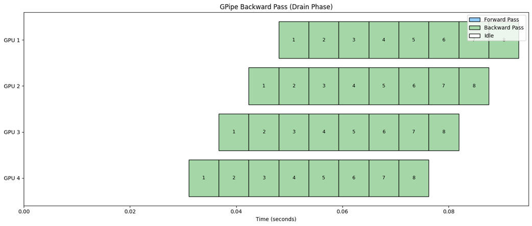
See how gradients move from the last GPU toward the first and leave idle time as the pipeline drains. section 6.5.3