A prediction error alone does not reveal which parameters caused it. Backpropagation traces the loss backward through a neural network, calculating how sensitive the loss is to each weight and bias. These sensitivities, or gradients, indicate the direction and rate of loss change as each parameter changes. section 11.2.4
The method applies the chain rule to the operations connecting a parameter to the loss. For an intermediate quantity z and prediction ŷ, ∂L/∂z = (∂L/∂ŷ)(∂ŷ/∂z): the local effects multiply to give the overall sensitivity. The backward pass reuses values from the forward pass and proceeds from the output toward the input. section 11.2.4 section 11.3.4
Figure 11.1 A simplified feedforward neural network containing an input layer, two hidden layers, and an output layer. Information moves forward through weighted connections to produce a prediction. During training, error information moves backward so that the weights and biases can be adjusted. Modern deep networks typically contain many hidden layers and many nodes within each layer, producing millions or even billions of adjustable parameters. Despite that scale, they follow the same basic forward-and-backward process shown here.
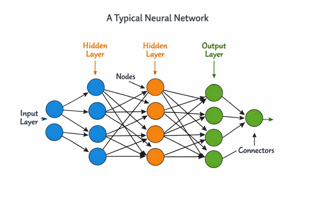
The diagram contrasts the forward flow of predictions with the backward flow of error information through a multilayer network. section 11.2
Backpropagation computes gradients; it does not update parameters. An optimizer such as gradient descent uses the gradients to make incremental adjustments. Training repeats prediction, loss calculation, gradient computation, and updating across mini-batches and epochs. Once training is complete, new predictions require only a forward pass. section 11.2.4 section 11.2.6 section 11.2
Pedestrian detection
Suppose a network predicts a pedestrian probability of 0.68 when the observed outcome is 1. Its cross-entropy loss is approximately 0.39. With a sigmoid output, the output-layer error signal is δ₀ = ŷ − y = −0.32; increasing the output score would reduce the loss. For a hidden-node output of 0.75, the connected output-weight gradient is δ₀ × 0.75 = −0.24. After gradient descent updates the parameters, the probability rises to about 0.69 and the loss falls to 0.37, although the braking decision remains unchanged. section 11.3.3 section 11.3.4 section 11.3.6
The same learning cycle applies to transformers: differentiable self-attention operations allow error signals to pass backward through attention projections and other components. Reducing training loss, however, does not guarantee good performance on unseen observations. section 12.3.1 section 10.5.1