Backpropagation computes how a model’s loss changes with each learnable parameter. A loss measures the difference between a prediction and its target; the resulting gradients guide small parameter adjustments intended to reduce that loss. section 8.2.1
In the forward pass, a computational graph connects inputs and parameters to a prediction and then to a loss. The backward pass starts at the loss and applies the chain rule through the graph, combining local gradients to find each parameter’s effect on the loss. Computing gradients is distinct from updating parameters. section 8.2.1 section 8.2.3
Figure 8.8 Prior to backpropagation, our model makes a prediction, and this prediction is compared to the actual target to compete the error. To figure out which parts of the graph contributed most to the error, we start from the end (the error) and work backwards through the solution process. The error is propagated backwards through the network and the contribution of each parameter (weight and bias) to the error is calculated. These parameters are adjusted slightly to reduce the error.
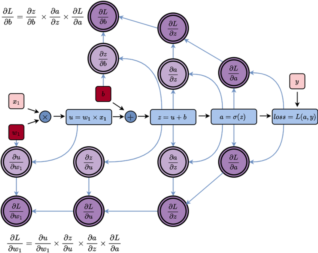
Follow the loss backward through a logistic regression graph to see how weights and bias contribute to the error. section 8.2.1
A PyTorch training step follows this sequence for each batch:
- Call optimizer.zero_grad() to reset parameter gradients, then compute predictions with model(inputs) and a loss with criterion(outputs, targets). section 8.2.3
- Call loss.backward() to calculate loss gradients for parameters with requires_grad=True. section 8.2.3
- Call optimizer.step() to update the parameters using those gradients. The learning rate scales the size of adjustments. section 8.2.3 section 8.2.1
Listing 8.5 Logistic Regression Model Class
x = torch.tensor([1.0, 2.0, 3.0])
w = torch.tensor([0.1, 0.2, 0.3], requires_grad=True)
b = torch.tensor(0.1, requires_grad=True)

z = torch.sum(x * w) + b
y = torch.sigmoid(z)

target = torch.tensor(1.0)
loss = torch.binary_cross_entropy(y, target)

loss.backward()
print(f"Gradient of w: {w.grad}")
print(f"Gradient of b: {b.grad}")
Try a small logistic regression calculation: the listing computes binary cross-entropy loss, runs loss.backward(), and prints the weight and bias gradients. section 8.2.1
Repeat the training step over batches and epochs. For validation, switch to model.eval() and use torch.no_grad(): validation calculates loss without updating the model or computing gradients. section 8.2.3