Correlation measures the direction and strength of a linear relationship between two continuous variables. Its coefficient ranges from -1 to +1: positive values mean variables move together, negative values mean they move in opposite directions, and values near 0 indicate no meaningful linear association. section 2.5.4
Read a coefficient as a quick description of linear association:
- Near +1: a strong positive relationship; as one variable rises, the other tends to rise. section 2.5.4
- Near -1: a strong negative relationship; as one variable rises, the other tends to fall. section 2.5.4
- Near 0: no meaningful linear relationship. As rough guides, values beyond ±0.8 are strong and values from ±0.6 to ±0.8 are fairly strong. section 2.5.4
- A strong correlation does not establish that one variable influences the other: correlation is not causation. section 2.5.4
Compute correlations only for numeric, continuous variables. In R, base `cor()` calculates a coefficient for two variables or a matrix for many variable pairs; use `use = "complete.obs"` to ignore missing values rather than receive `NA`. Pearson correlation is the default for linear relationships, while Spearman uses ranked values and is interpreted on the same -1 to +1 scale. section 10.4.1 section 2.5.4
From a matrix to a heat map
For draft variables Age, games, minutes played, Win Shares, and Win Shares per 48 minutes, select the numeric columns, run `cor()`, reshape the matrix, and map coefficients to tile colors. The displayed matrix makes many pairwise relationships readable at once: games and Win Shares correlate about 0.80, while Age and Win Shares correlate about -0.25. section 2.5.4
Figure 2.4 Matrix of correlation coefficients between all continuous variables in the draft data set
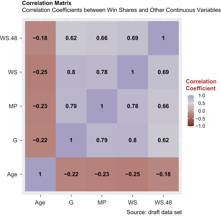
Use the correlation matrix to compare every numeric-variable pair at once, with color and rounded labels exposing direction and magnitude. section 2.5.4
A scatterplot, or correlation plot, shows one numeric variable on each axis. Add `geom_point()` for observations and `geom_smooth(method = lm)` for a linear regression line; the line summarizes the trend, while the coefficient supplies its numeric strength and direction. For example, annual salary and win shares have a positive, strong correlation of about 0.76. section 4.5.3
Correlation can screen candidate predictors before linear regression, especially in wide data sets. Compare each variable with the target rather than automatically including every independent variable, but treat the result as an association check—not proof of influence. A deflections–wins coefficient of 0.24, for instance, is positive but unremarkable. section 5.6 section 5.6.1
Compare offense and defense
Standardized points allowed and wins correlate -0.58, while standardized points scored and wins correlate 0.53. Although points allowed has the larger absolute correlation, the difference is negligible, so these results do not support a material defensive advantage for regular-season wins from 2008 through 2017. section 14.4.1















