Suppose you know the prices of several houses and want to estimate the price of one more. Linear regression looks for a straight-line pattern between a numerical feature, such as the number of rooms, and a numerical target, such as price. It is a supervised learning method: the known houses provide both features and prices. Unlike classification, which predicts a category such as spam or not spam, regression predicts a number. section 2.2 section 3.2
A price from the number of rooms
Imagine that each additional room adds $50 to a base price of $100. The model is Price = 100 + 50 × (number of rooms), so it predicts $300 for a four-room house. The $50 is the feature’s weight, also called the line’s slope; the $100 is the bias, or intercept. Real prices need not fall exactly on the line: the goal is a useful estimate, not a perfect match for every house. section 3.2 section 3.3
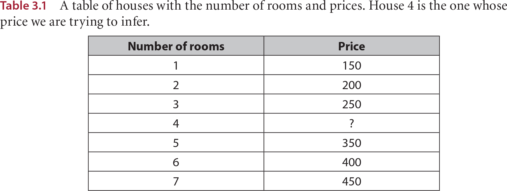
Table 3.1 A table of houses with the number of rooms and prices. House 4 is the one whose price we are trying to infer. (view table figure)
| Number of rooms |
Price |
| 1 |
150 |
| 2 |
200 |
| 3 |
250 |
| 4 |
? |
| 5 |
350 |
| 6 |
400 |
| 7 |
450 |
The house-price table makes the missing four-room price a prediction you can try before using the formula. section 3.2
Plot room count horizontally and price vertically. Each known house becomes a point; fitting the model means placing a line close to the points. With several features, the prediction is a bias plus a separate weight times each feature—for example, room count, size, school quality and age. The one-feature picture is easier to draw, but the same weighted-sum idea extends to those additional inputs. section 3.0 section 3.2
One way to fit the line is to improve it repeatedly:
- Start with a random slope and intercept, then select a data point. section 3.3
- Compare the line’s predicted price with that point’s actual price. Use the difference to adjust the slope and intercept; a learning rate scales the adjustment. section 3.3
- Repeat for many iterations and use the resulting line to predict prices for new houses. section 3.3
Figure 3.6 An illustration of the linear regression algorithm. We start at the top left with a random line and end in the bottom left with a line that fits the dataset well. At each stage, two things happen: (1) we pick a random point, and (2) the point asks the line to move closer to it. After many iterations, the line will be in a good position. This figure has only three iterations for illustrative purposes, but in real life, many more iterations are needed.
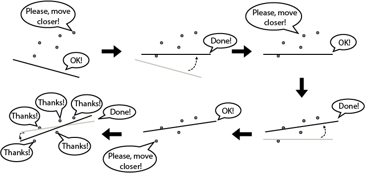
The diagram shows how successive adjustments move an initial line toward the data points. section 3.3
On a real housing dataset, a fitted line needs checking. A Turi Create example loads 6,207 Hyderabad houses, trains a model to predict Price, and reports root mean square error (RMSE). Its RMSE is about 3,000,000 in the dataset’s price units; outliers and missing price-relevant features are possible concerns. You can also train using only Area, inspect the coefficient and intercept, and plot the resulting line. If the pattern calls for a curve rather than a line, polynomial regression is an alternative. section 3.5 section 3.9
Try plotting a small set of house sizes and prices. Guess a line, use it to predict a withheld price, then compare the prediction with the known value. Which points lie farthest from your line? section 3.2 section 3.3