Linear regression predicts a numeric outcome from one or more inputs by fitting a straight-line relationship to observed data. Think of a retailer asking whether warmer days lead to more sports drink sales, or a real-estate company estimating a house price from square footage. The fitted line turns an input value into a predicted output value, provided a linear pattern is a reasonable assumption. section 1.0 section 7.0 section 7.6
For simple linear regression, one input x predicts one output y with y = mx + b. The slope m describes how much the prediction changes for each one-unit increase in x; the intercept b is the prediction when x is zero. A useful intercept is not guaranteed: it can fall outside a meaningful range even when the line predicts well within the observed data. section 7.7
Temperature and sports drink sales
Ten sampled days pair temperature with sales. A fitted slope of 9.74 means predicted sales rise by 9.74 for every additional degree Fahrenheit. The intercept, -405.26, would represent predicted sales at 0°F, but negative sales are not meaningful. Read coefficients in the context of the available data rather than treating every number as a practical claim. section 7.7
Figure 7.7 Using matplotlib to show a linear regression against our data
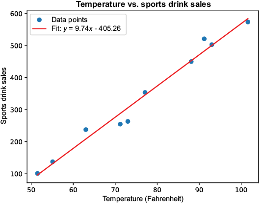
Compare the scatterplot with its fitted line to see the prediction pattern and the distance between observed points and model predictions. section 7.7
With several inputs, multiple linear regression gives each predictor its own slope. House square footage, lot square footage, and backyard square footage can each contribute a term. These slopes are often written as beta coefficients: β0 is the intercept, while β1, β2, and β3 are slopes for their respective inputs. The notation is fancier than the idea. section 7.11
A fitted line leaves residuals: the differences between actual and predicted values. Least sum of squares chooses coefficients that make the total of squared residuals as small as possible. Squaring prevents positive and negative misses from canceling out and supplies the basis for measures such as R² and root mean squared error (RMSE). Smaller RMSE means smaller residuals in aggregate, but a score alone is not a verdict. section 7.9 section 7.11
Use linear regression carefully:
- Plot the data and inspect it alongside numerical metrics; R² and RMSE can miss misleading patterns. section 7.11
- Avoid claiming causation from correlation or regression alone. section 7.13
- Do not extrapolate the fitted trend beyond the data range. section 7.13
- Check whether outliers and unequal variability undermine a linear relationship, and reconsider weak predictor hypotheses. section 7.13
- Use a different model when the outcome is binary; logistic regression fits probabilities with an S-shaped curve rather than an awkward straight line. section 8.2





















