A linear regression predicts a target as a linear combination of input features. For a demand forecast, it can be a useful step between a simple sales-based rule and a more specialized forecasting model. section 8.6.1 section 9.2.2
Start with a constant baseline, then try a rule-based baseline and a linear model. Compare the improvement in the chosen metric with the time and computing resources needed to implement, train, debug, and test each option. Interpretability and computation time matter too. A more complex model is worth pursuing only if the simpler alternatives are insufficient for the task. section 8.3 section 8.5
Retail demand forecasting
For each product and grocery, a constant baseline can predict sales using the actual value from one week earlier, accounting for weekly seasonality and possible data delays. A linear regression baseline can instead use quantile loss with lagged sales and rolling summaries, such as sums, averages, medians, and quantiles over several window sizes. Price or customer counts can provide additional dynamic features. section 8.6.1
After fitting a simple linear regression, inspect residuals for patterns that challenge its assumptions. Checks include linearity, zero-centered residuals, normality, constant residual variance, and independent errors. Influential outliers in predictors or targets can also cause problems. Unexpected patterns may suggest better features or an alternative model; important assumptions can also become tests that guard against unexpected behavior after deployment. section 9.2.2
Figure 9.10 Four diagnostic plots for linear regression’s residual analysis in both cases (Case 1: Assumptions are met)
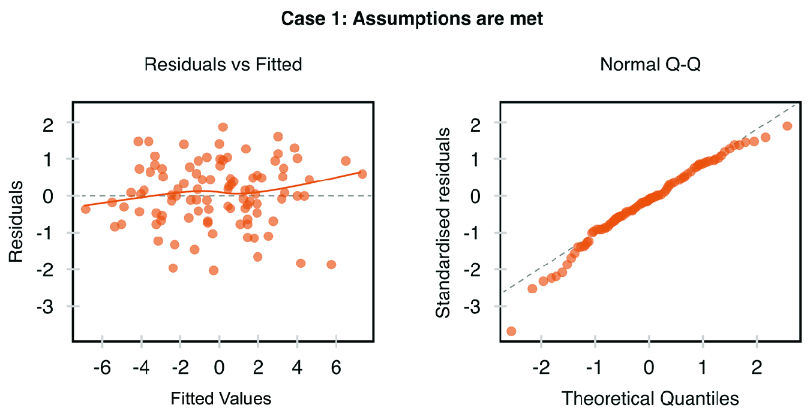
Compare diagnostic plots for a case where the regression assumptions are met with plots from a case where they are not. section 9.2.2
Figure 9.11 Four diagnostic plots for linear regression’s residual analysis in both cases (Case 2: Assumptions are not met)
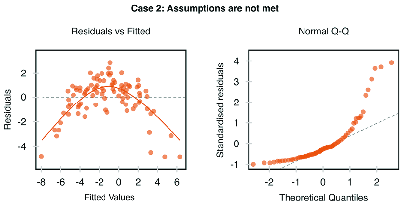
Use these plots alongside the assumptions-met case to spot diagnostic differences. section 9.2.2