Linear regression predicts a numeric response from one or more predictors by fitting a linear equation to observed data. It can also describe the direction and size of an association. Use it for quantitative outcomes, such as sales revenue or race split times—not for categorical classification. section 4.0 section 4.1
With one predictor, the prediction is ŷ = β₀ + β₁x: β₀ is the intercept and β₁ is the predicted change in the response for a one-unit change in x. An observed value may differ from ŷ by an error. Multiple linear regression adds a coefficient-weighted term for each additional predictor. Ordinary least squares (OLS) estimates the coefficients by minimizing the sum of squared differences between observed and predicted responses. section 4.1.1 section 4.2.2
A practical fitting workflow is:
- Explore the variables with scatterplots and correlation measures; check normality and investigate possible outliers before fitting. section 1.5.1 section 4.2
- Choose a numeric response and predictors, add an intercept, fit the model, and inspect its regression table. section 4.2.2
- Evaluate fit and coefficient significance, then test assumptions before relying on the results. section 4.3 section 4.2.4
Predict a race split
To estimate Stage 2 ultramarathon split time from Stage 1 split time, fit: `y = mds['stage2']; x = sm.add_constant(mds['stage1']); lm = sm.OLS(y, x).fit(); print(lm.summary())`, after `import statsmodels.api as sm`. The resulting table reports an R² of 0.575 for 20 observations. Fitting is quick; deciding whether its predictions are trustworthy requires interpreting the table and checking assumptions. section 4.2.2
R² gives the proportion of response variance explained by the model, but it does not establish linearity or, alone, settle model quality. Check the overall F-statistic and p-values for individual coefficients. A low R² calls for examining explained and total variation rather than automatically adding predictors, which can increase complexity and multicollinearity. section 4.3 section 1.4.1
Figure 4.7 A residuals plot that displays the fitted values from a linear regression on the x axis and the residuals from the same model on the y axis. Linearity between variables is confirmed when the data points do not follow any obvious pattern or trend.
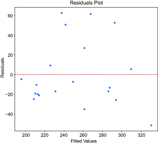
A fitted-values-versus-residuals plot helps check linearity: points scattered without an obvious pattern support a linear model, while a pattern suggests unexplained structure. section 4.2.4
Also check residual independence, constant variance (homoscedasticity), and residual normality before treating the output as reliable. Outliers can strongly affect fit. Transformations may help with skewed data, but they change the scale on which the modeled relationship is interpreted and should not substitute automatically for considering a different model. section 4.2.4 section 4.1.3





















