The mean, or expected value, is a single-point summary of a probability distribution. Imagine drawing samples repeatedly: values with higher probability occur more often, so the long-run average is pulled toward them. With sufficiently many samples, that average settles near a fixed distribution-specific value, written μ. The mean need not be a value that any individual draw can produce; it summarizes the whole distribution rather than predicting one outcome. section 5.7.1 section 5.10
For a discrete random variable X taking values xi with probabilities p(xi), the mean is the probability-weighted sum E[X] = Σi xi p(xi). For a continuous variable, replace the sum with an integral: E[X] = ∫ x p(x) dx. A multivariate random variable has a mean vector, obtained by taking the probability-weighted average of its vector-valued samples. More generally, E[f(X)] weights each possible value of a function f by the probability of its input. section 5.7.1
Geometrically, the mean is a centroid. Treat probability at each location as mass: the mean is the one point that balances the distribution. This also clarifies its relationship with variance. Variance measures the expected squared distance from μ, so it describes whether samples cluster tightly around the center or spread far from it. In several dimensions, covariance extends this idea by recording spread and joint variation across directions. section 5.7.1 section 5.7.2
Means play several practical roles in probabilistic machine learning:
- Parameterize a Gaussian: μ sets the center, or most likely location, of its bell-shaped density; in the multivariate case, μ is a vector. section 5.9.2
- Estimate an unknown Gaussian from data: maximum likelihood uses the sample mean as the estimated mean parameter. section 6.8.1 section 13.2
- Combine data with prior belief: Bayesian estimation updates a prior mean toward the sample mean, with data having greater influence as sample size grows. section 13.3
- Locate mixture components: each Gaussian mixture component has its own μk, which determines its density peak and sample-cloud centroid. section 6.9.1
- Represent inputs in a VAE at inference time: a Gaussian encoder emits a mean and covariance, and its mean is used directly as the latent representation. section 14.7.1
Sample mean versus a distribution mean
Suppose a Bernoulli trial is encoded as 1 for success and 0 for failure, with success probability π = 0.3. The mean is 0.3: across many trials, the average encoded outcome approaches 0.3, even though one trial produces only 0 or 1. Likewise, for a binomial variable counting successes in n trials, the expected count is nπ; with 100 trials and π = 0.2, it is 20. These are long-run weighted averages, not fractional single-trial outcomes. section 5.9.5 section 5.9.3
Figure 5.10 Gaussian densities with varying μs and σs. Changing μ shifts the center of the curve. A larger σ (variance) implies a fatter bell ⇒ more spread. Note that fatter curves are smaller in height as the total area under the curve must be 1.
|
(a) Different μs but the same σs. |
|
(b) The same μs but different σs. |
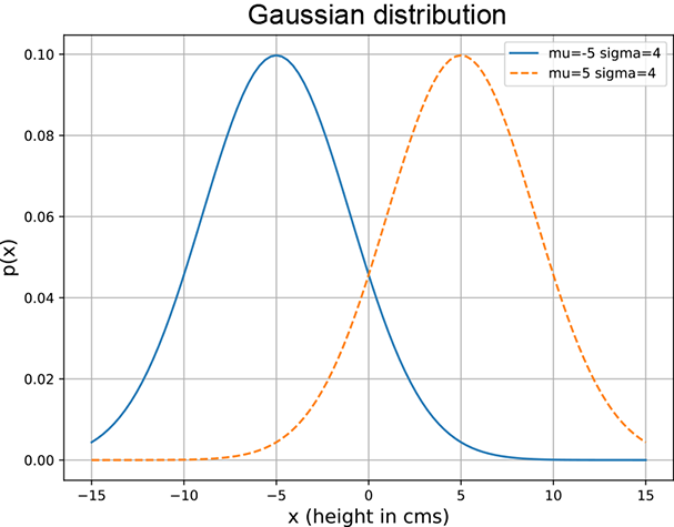
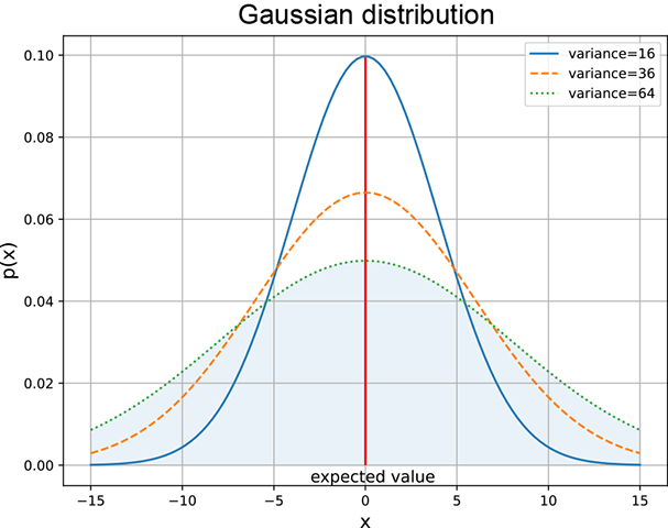
Compare Gaussian curves while changing μ: shifting μ moves the density's center, whereas changing σ alters its spread. section 5.9.2