A classifier learns to assign an input to one of K discrete classes. Given labeled training pairs D = {(xᵢ, yᵢ)}, it learns a rule h that predicts a label for a new input. K = 2 gives binary classification; K > 2 gives multiclass classification. Unlike regression, the target is a class rather than a continuous value. section 5.1 section 1.1
Often the input first becomes a d-dimensional feature vector φ(x), giving a prediction h(φ(x)). The goal is not merely to match training labels: the rule must generalize to unseen examples. One direct loss is the misclassification rate, (1/n)∑ᵢ 1[h(φ(xᵢ)) ≠ yᵢ], where the indicator is one for a mistake and zero otherwise. Training seeks parameters that reduce loss; model selection also checks whether the chosen capacity underfits or overfits. section 1.1 section 5.1
Several classifiers implement this mapping in different ways:
- A perceptron uses a linear decision boundary, θ·x + θ₀ = 0, and updates it when a labeled example is misclassified. section 5.2 section 5.8
- A support vector machine seeks a maximum-margin boundary; training points on its margins are support vectors. Logistic regression computes class conditional density using a softmax function. section 5.8
- Bernoulli naive Bayes represents each document word as present or absent. It assumes features are conditionally independent given the class, so their class-conditional density factors into one-dimensional terms. section 5.5
- A CART classification tree recursively chooses feature thresholds to partition the input space. A leaf predicts by majority vote; split costs such as Gini impurity favor purer leaves, while limiting depth helps prevent overfitting. section 5.6
For binary predictions, a confusion matrix separates true positives, true negatives, false positives, and false negatives. Changing the classification threshold changes these counts. ROC curves plot true-positive rate against false-positive rate across thresholds; precision–recall curves provide another view of performance. section 5.2
Document classification with Bernoulli naive Bayes
Convert each document into indicators xᵢⱼ: 1 if word j occurs in document i, otherwise 0. Estimate class and word-presence parameters from labeled documents, then compare class scores for a new document under the conditional-independence assumption. An implementation uses tokenization, stop-word filtering, and the 20 Newsgroups dataset. section 5.5
Figure 5.1 Model selection to avoid overfitting or underfitting to training data
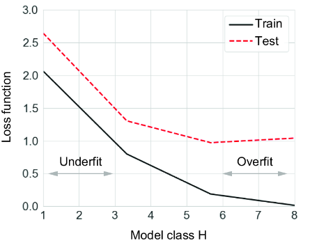
Compare training and test loss as model capacity changes to see where a classifier underfits or overfits. section 5.1