A classifier maps an input to one class from a predetermined set. A face detector, for example, maps an image to face or not face; a multiclass system might choose cat, dog, airplane, or automobile. Classification differs from regression: regression emits a numeric estimate, while classification emits a decision or category. A model may produce the class directly, or convert a score into classes by thresholding it. section 1.5 section 7.2.2 section 1.3.2
Geometrically, each input is a point in a feature space. A classifier divides that space into regions for different classes; the separating surface is the decision boundary. For binary classification, evaluating the boundary function at an input determines its side of the boundary, and the sign can determine the predicted class. A linear classifier uses a hyperplane, but real class regions may require curved boundaries. section 3.8 section 3.1.4 section 1.4
Training a classifier turns labeled examples into a decision rule:
- Collect training inputs paired with ground-truth class labels; manually creating these labels is often difficult. section 3.1.3
- Choose a parametric function family, using a linear model for simple cases or a nonlinear model for more complex ones. section 3.1.3
- Adjust parameters iteratively to reduce loss between model outputs and known labels; gradients indicate parameter adjustments that reduce loss. section 3.8
- During inference, evaluate the trained function on a new input and select its class, by a sign, threshold, or highest-scoring output as appropriate. section 1.3.6 section 9.2.3
From height and weight to three classes
A neural classifier can take height and weight as inputs and predict man, woman, or child. Two linear layers produce three raw scores. During training, PyTorch CrossEntropyLoss receives those raw scores and the class labels; during prediction, softmax converts scores to class probabilities and argmax selects the predicted class. Minibatches, gradient computation, and SGD update the weights over training epochs. section 9.2.3
Neural networks extend classifiers beyond linearly separable data. A perceptron creates a linear boundary, so it can separate two half-spaces but cannot represent curved class regions. Multilayer perceptrons combine perceptrons to construct more complex regions; for instance, several boundary tests can be ANDed to recognize a rectangular region. With sufficient perceptrons, polygonal regions can approximate shapes on a plane. section 7.6 section 7.5.4
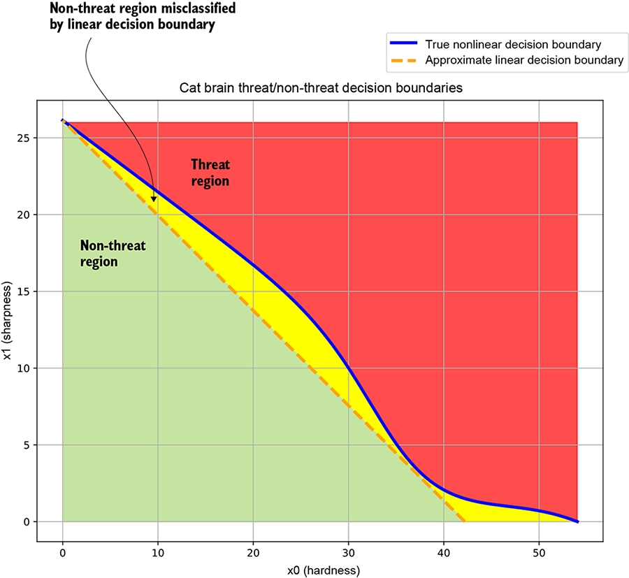
Figure 7.4 Classifiers, decision boundaries, and training data. Data points from different classes are marked with different symbols (plus and dot).
|
(a) Cat brain threat model decision boundary. The solid curve corresponds to the true decision boundary separating the threat and non-threat regions. The dashed line represents an approximate linear decision boundary: it classifies most points correctly but misclassifies points in the region between itself and the true decision boundary. |
|
(b) Good training data. Sample points from each class roughly span the region of input space belonging to the class. This yields a good decision boundary (solid line). |
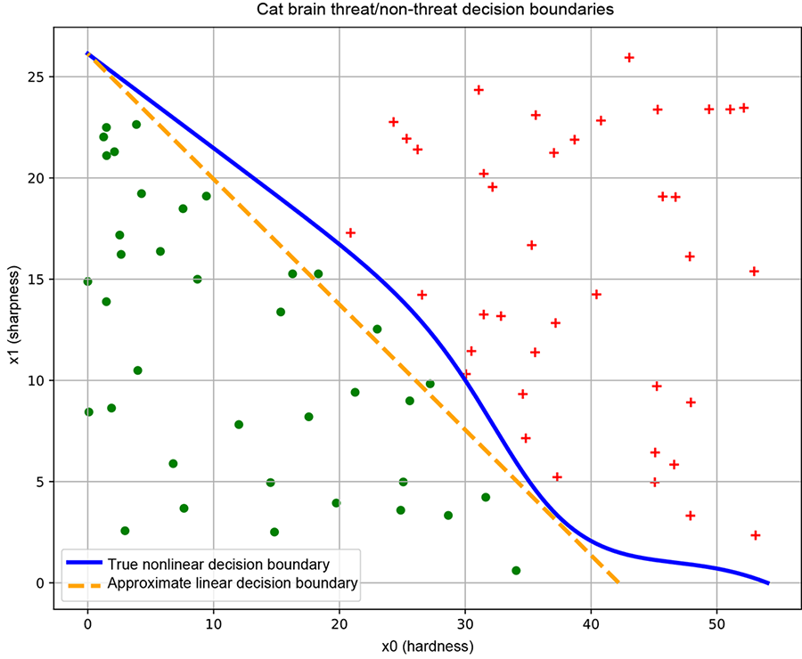
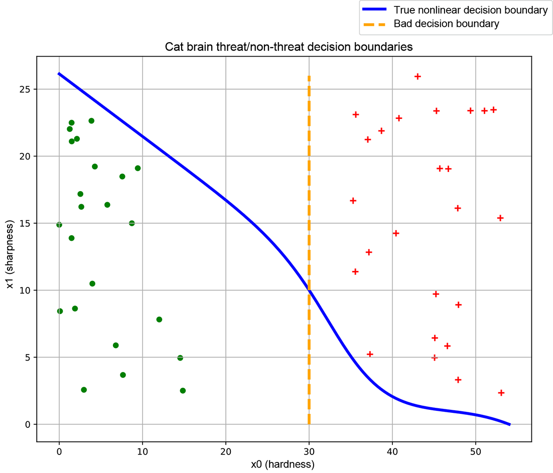
Compare representative training points with the resulting good and bad decision boundaries to see why coverage of each class region matters. section 7.2.2
Image classification applies the same mapping to pixels: a classifier can assign an image a digit label or one or more object categories. Convolutional neural networks make this practical by learning features rather than relying on hand-crafted rules. In object detection, a classifier is paired with a regressor: classifier layers assign a class to each region of interest, while regression layers predict bounding-box coordinates. section 11.1 section 11.0 section 11.4.3