Suppose today could bring no rain, 0.01 inches per hour, or 0.02 inches per hour. A mean summarizes these possibilities in one number. When the possibilities have different probabilities, use a probability-weighted average, also called an expected value: multiply each value by its probability, then add the results. section 1.5
A mean rainfall rate
If the three rainfall rates have probabilities 0.8, 0.1, and 0.1, the mean is 0(0.8) + 0.01(0.1) + 0.02(0.1) = 0.003 inches per hour. An ordinary average of the three rates would be 0.01, but it would ignore how much more likely no rain is. The mean need not be a value that actually occurs. section 1.5
A mean also locates the center of a normal distribution. For a normal prior centered at $100 per square foot, the mean expresses an initial estimate of a house-price slope; the standard deviation expresses uncertainty around it. After observing prices, the posterior mean moves toward the value supported by the data, while a smaller posterior standard deviation reflects reduced uncertainty. In Python, the updated mean is calculated from the prior mean and variance together with the observed features, prices, and noise variance. section 3.12 section 3.14
Figure 3.6 The posterior predictive distribution of individual datapoints in the test set, illustrated by the predictive mean and 95% credible intervals. Most datapoints in the training set falls within the credible intervals.
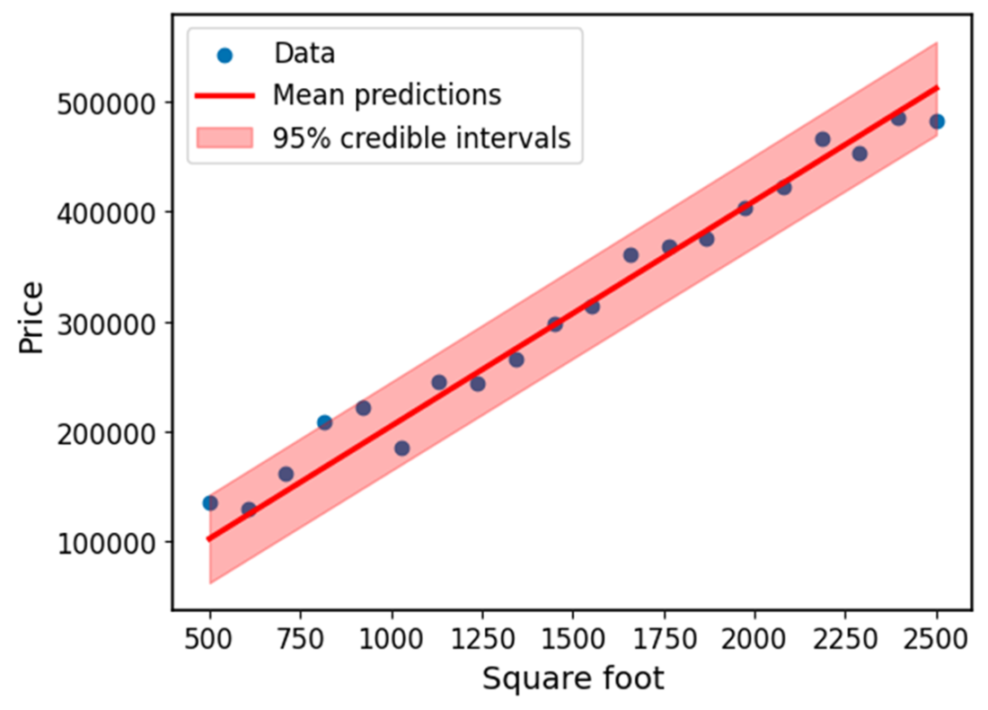
The prediction line shows mean house prices; credible intervals show the uncertainty that a line of means alone would hide. section 3.15
A useful mean still needs context. In variational inference, a normal approximation has a mean describing its center, but its symmetric shape may not match an asymmetric posterior perfectly. In a decision, the quantity being averaged can instead be a payoff: multiply each possible gain or loss by its probability and compare the expected values of the available actions. section 6.3 section 11.10
Should a new design launch?
A launch gains $100,000 with probability 0.97 and loses $20,000 with probability 0.03. Its expected gain is $100,000(0.97) − $20,000(0.03) = $96,400, versus $0 for doing nothing. If the possible loss rises to $4 million, the expected gain becomes −$23,000. The probabilities have not changed, but the decision has. section 11.10