Linear regression models a response as a line through one or more predictors. For a house, square footage is the predictor and price is the response: y = mx + b. The slope m describes how the predicted price changes with area; the intercept b shifts the line. Starting with b = 0 keeps the first calculation simple. section 3.10
A useful line makes small errors on historical data. One closed-form calculation chooses the slope that minimizes average squared error, then uses that slope to predict prices for unsold houses. A single best-fit value can mislead when data are scarce or noisy: two points can determine a perfect line even when future predictions remain uncertain. section 3.10 section 3.11
Bayesian linear regression keeps a probability distribution over the slope instead of committing to one value. A prior expresses an initial belief, and observed data update it to a posterior. With a normal prior and normally distributed noise, the posterior remains normal, so its mean and uncertainty can be calculated directly. section 3.11 section 3.13
Updating a house-price slope
Suppose the unknown slope initially follows N(100, 100²), while noise has mean zero and standard deviation 20,000. Synthetic data use a true slope of 200, square-footage values from 500 to 2,500, and noisy prices. After updating, the posterior mean moves near 200 and its standard deviation shrinks. This lets you ask whether each square foot is worth more than $200 or at most $190 on average. section 3.13 section 3.14
The model extends in several practical directions:
- Use multiple predictors—such as stories, location, and construction date—with a weight for each feature. section 3.16
- Use a stronger prior to pull weights toward a preferred value when data are sparse or noisy, paralleling regularization. section 3.16
Figure 3.5 The prior and posterior distributions of the slope 𝑚. The posterior distribution sharply peaks around the true value 𝑚 = 200 to reflect the insight from the observed data.
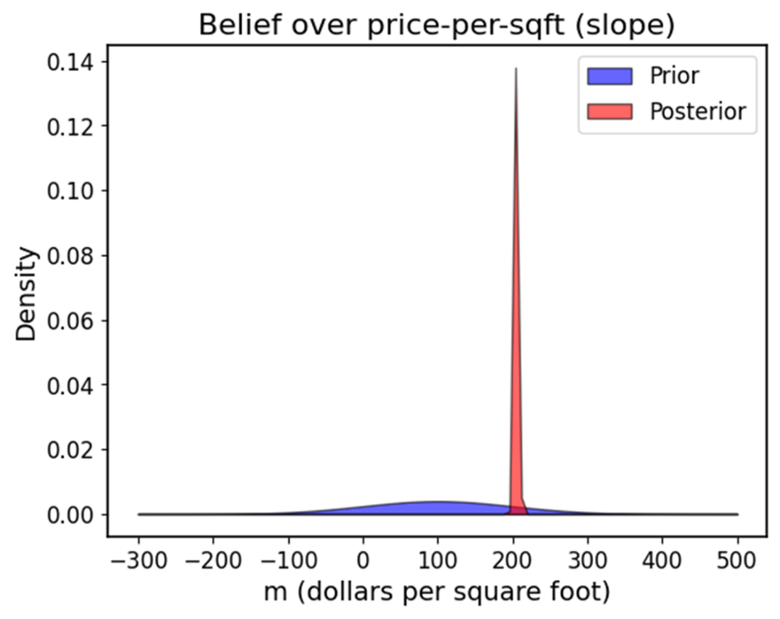
Compare the prior and posterior slope distributions to see how data concentrate belief around the true value. section 3.14