A probability distribution describes how values are apportioned across possible outcomes. In tabular data, a single-feature distribution describes one column; a joint distribution describes how values of two or more features occur together. Both matter when deciding what is typical. section 11.2.2
For outlier detection, training rows must be typical, but that is not enough: their proportions should also reflect the population. Overrepresenting one segment can shift estimated means and standard deviations, distort apparent distances and sparse regions, and make an unreliable pattern seem normal. section 4.4 section 4.15
The distribution needed depends on the task:
- To screen a numeric column for extreme values, statistical tests describe its spread using quantities such as standard deviation or interquartile range. Check their assumptions: simple tests often work on one column and may expect an approximately Gaussian distribution. section 2.0
- To generate synthetic rows, a histogram or kernel density estimate can approximate each feature’s observed distribution. Drawing columns independently may reproduce each column’s values while losing relationships between columns; generating later features from earlier ones can preserve more of those relationships. section 11.2.2
- To compare groups, express each category’s count as a fraction of its group total and put categories in the same order. This compares distribution shapes rather than group sizes. Visual plots can be supplemented with a distance such as Jensen–Shannon distance. section 12.8
Figure 11.2 The distribution of At_bats is shown in the left pane for both the real and synthetic data. The distributions are almost identical. The middle pane shows the joint distribution of At_bats and RBIs in the real data, and the right pane shows the same two features in the synthetic data. The relationship between these features is not maintained in the synthetic data.
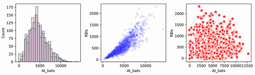
Compare the single-feature plot with the two-feature plots: similar distributions of At_bats do not imply that the At_bats–RBIs relationship survives independent generation. section 11.2.2
Supplier use by purchaser
Plot supplier frequencies for all purchasers and for each purchaser. Overall comparisons show no clearly unusual pattern; restricting the data to purchases on day 28 makes one purchaser’s supplier distribution stand out. The narrower context changes what can be seen, but a visible difference still requires interpretation before it is treated as an anomaly. section 12.8
Figure 12.8 Looking only at purchases on the 28th day of the months: distributions of suppliers used for the full dataset (top left pane), and for staff 0, 1, and 10 in the other plots. Staff 10 (bottom right pane) stands out as having an unusual distribution relative to the other staff. It may explain the unusual shape of the full dataset, which also has a spike for supplier 10.
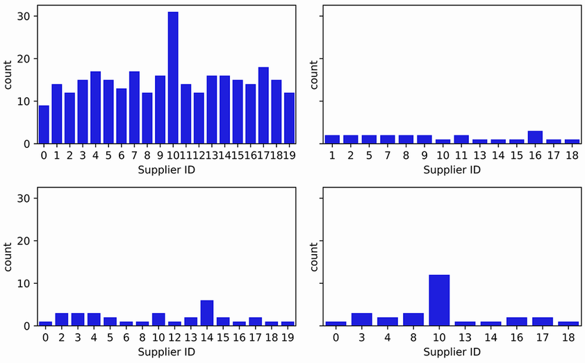
The day-28 plots show why comparing distributions within a relevant subset can reveal a difference that broader plots do not make obvious. section 12.8