Suppose you need to search a long list. Checking entries one by one may feel quick when the list is short—but what happens when it grows to a billion entries? To compare algorithms at different sizes, count how their operations grow rather than timing one run in seconds. Big O notation names that growth rate. section 1.5 section 1.10
A small test can mislead you
If checking an entry takes 1 ms, simple search needs up to 100 ms for 100 entries; binary search needs about 7 ms. With a billion entries, the estimates become a billion milliseconds—about 11 days—for simple search and about 30 ms for binary search. The gap does not stay fixed as the list grows. section 1.7
Let n be the input size. Simple search is O(n): in the worst case, it checks every entry. Binary search is O(log n): its number of steps grows much more slowly. For a list of four billion items, their maximum counts are four billion checks and 32 guesses, respectively. section 1.5 section 1.9
Try it with paper
To make a grid of 16 boxes, drawing each box takes 16 operations, or O(n). Folding paper so each fold doubles the number of boxes takes four operations, or O(log n). The steps you choose change how the work grows. section 1.8
Common running times, from faster-growing work to slower-growing work as inputs increase, are:
- O(log n): binary search. section 1.10
- O(n): simple search. section 1.10
- O(n × log n): a fast sorting algorithm such as quicksort. section 1.10
- O(n²): a slower sorting algorithm such as selection sort. section 1.10
- O(n!): a traveling-salesperson algorithm. section 1.10
A lucky search can finish on the first entry, but that does not change simple search’s O(n) worst-case label. Average-case time is worth considering too. Nor does a Big O label convert neatly into an exact operation count or number of seconds. section 1.9 section 1.10
The same idea applies beyond lists. Breadth-first search follows graph edges and queues people to search, giving O(V+E) time: V for vertices and E for edges. section 6.8
Run times grow at very different speeds!
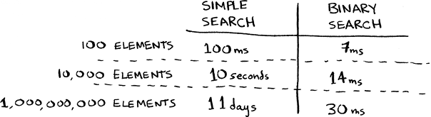
Compare how the running times of simple search and binary search diverge as the list grows. section 1.7