A search that feels quick on ten items may feel very different on a million. Performance describes the resources an algorithm or data structure uses, especially running time and memory. The useful question is not just “Which is faster?” but “How will its costs change as the input grows?” section 4.1 section 4.7
There are two complementary ways to answer that question:
- Profile an implementation: run the code on various inputs and measure its time and memory. This helps find bottlenecks after implementation. section 4.1 section 4.4
- Analyze the algorithm: reason about how time and space grow with input size, often using big-O notation. This helps compare options during design without relying on one particular implementation. section 4.3 section 4.4
Big-O gives a growth bound, not an exact stopwatch reading. O(1) is constant growth, O(log(n)) is logarithmic, and O(n) is linear. Constant factors and smaller terms can be dropped when describing growth: 3n + 5 is O(n). An estimate from this model can reveal whether an approach is likely to remain practical at a larger scale, but it does not report the actual running time of your code. section 4.16 section 4.10 section 4.9
Searching an array
In the worst case, linear search scans all n elements, so its running time is O(n). Binary search repeatedly halves the remaining range, giving O(log(n)) time and O(1) extra space—but it requires a sorted array. If you need many searches, that prerequisite is worth considering before choosing between them. section 4.14 section 4.15
Time is only one cost. Reversing an array into a second array needs O(n) extra space; swapping elements in place needs O(1). For any operation, ask whether you mean its worst case, its expected cost across possible inputs, or its amortized cost across a sequence of operations. A single slow operation need not make the whole sequence equally slow. section 4.12 section 4.11
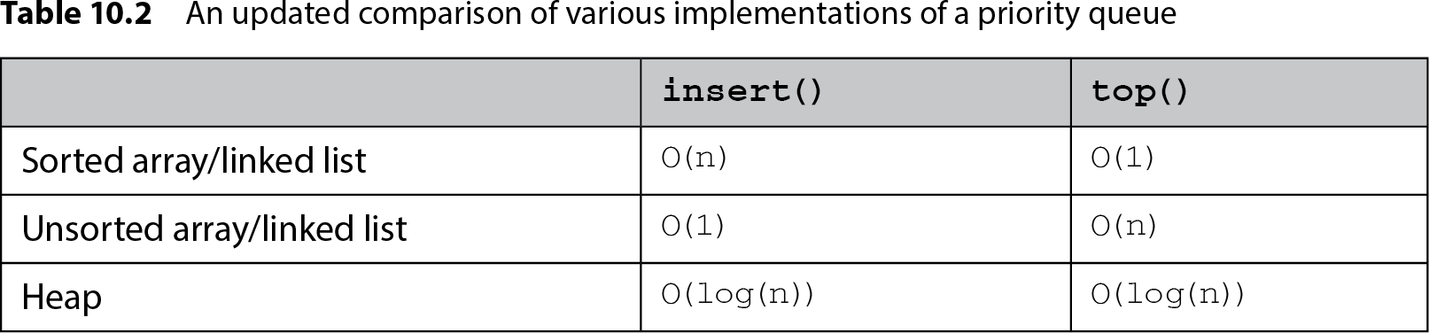
Table 10.2 An updated comparison of various implementations of a priority queue (view table figure)
| insert() |
top() |
|
|---|---|---|
| Sorted array/linked list |
O(n) |
O(1) |
| Unsorted array/linked list |
O(1) |
O(n) |
| Heap |
O(log(n)) |
O(log(n)) |
Compare priority-queue implementations by operation, not by a single verdict: sorted and unsorted collections trade fast insert for fast top, while a heap offers O(log(n)) for both. section 10.12
A practical routine is to identify the operations a solution needs, compare their time and space costs, then implement and profile the choice. Keep the requirements in view: a working solution can still be too slow or use too much memory, while the theoretically best option may not be necessary. section 1.9 section 4.4