A normal distribution, often called a bell curve, represents uncertainty about one quantity. Its mean gives the expected value and its variance gives the spread. In Gaussian-process prediction, this turns a single estimate into a distribution: the center is the predicted value, while the range expresses confidence. Predictions near observations can be more certain than predictions far away. section 2.0 section 2.6
Estimating a house price
Before seeing comparable sales, a homeowner may believe a house is worth roughly $150k–$300k. A nearby, similar house sold for $250k shifts that belief toward a narrower $230k–$270k range; an unrelated California sale need not change it. The normal distribution captures both the estimate and the remaining uncertainty. section 2.1 section 2.2.2
For several quantities at once, use a multivariate Gaussian distribution. Its mean vector contains the expected value of each variable. The covariance matrix places each variable’s variance on the diagonal and records relationships between variables off the diagonal. Strong positive correlation means observing one variable can shift the mean and reduce uncertainty for another; weak correlation leaves it largely unchanged. section 2.2.1 section 2.2.2
Conditioning updates a Gaussian belief after an observation:
- Fix the observed variable at its known value; its posterior uncertainty becomes zero. section 2.2.2
- Update correlated variables’ means and variances, with stronger effects for stronger correlations. section 2.2.2
- Leave uncorrelated variables essentially unchanged by that observation. section 2.2.2
Figure 2.4 An MVN distribution groups multiple normally distributed random variables together. While the mean vector of the MVN concatenates the mean values, the covariance matrix models the correlations between the individual variables.
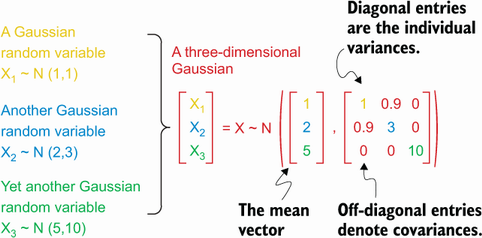
Use the mean vector and covariance matrix diagram to distinguish individual normal distributions from their joint multivariate model. section 2.2.1
A Gaussian process extends this idea from a finite vector to function values across an input domain. Every finite set of function values follows a multivariate Gaussian, so a model can make normal-distribution predictions at individual test points while using covariance to connect similar inputs. These predictive distributions support Bayesian optimization, where possible improvement over the current best value is assessed from the distribution at each candidate point. section 2.3 section 4.2.1