The normal, or Gaussian, distribution models a continuous quantity that is most likely near a center and progressively less likely farther away. Its probability density is a symmetric bell: it peaks at the mean μ, approaches zero without reaching it, and assigns equal density to equally distant values on either side of μ. The notation 𝒩(x; μ, σ²) names a univariate Gaussian, where μ locates the bell and σ controls its width. section 5.9.2
Figure 5.7 Univariate Gaussian random probability density function, μ = 0 and σ = 4. The bell-shaped curve is highest at the center and decreases more and more as we move away from the center, approaching zero asymptotically. The value x = 0 has the highest probability, corresponding to the center of the probability density function. Note that the curve is symmetric. Thus, for instance, the probability of a random sample being in the vicinity of −5 is the same as that of 5 (0.04): that is, p(−5) = p(5) = 0.04. An interactive visualization (where you can change the parameters and observe how the graph changes as a result) can be found at http://mng.bz/NYJX.
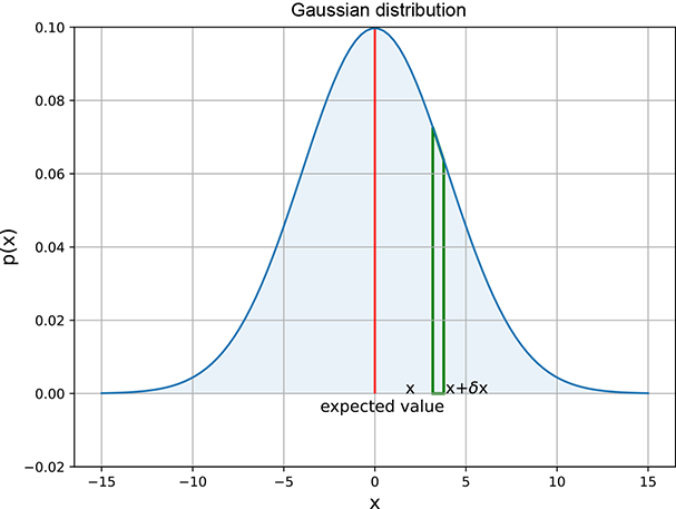
Use the bell curve to inspect symmetry, the central peak, and the gradual fall in density away from μ. section 5.9.2
Width expresses spread: increasing σ makes the bell wider and lower because its total area must remain 1. Consequently, a wider Gaussian is less peaked and has higher entropy. The expected value is the center of the bell, while variance quantifies its spread. section 5.9.2 section 6.2.2
Adult heights and weights
If adult weights cluster around 75 kg, a Gaussian places its greatest density near 75 and smaller density at 70 or 80; distant values such as 40 or 110 are unlikely. Likewise, observed female heights can fit a Gaussian: estimate μ and σ from samples, then compute the probability of a height falling between 160 and 170 cm. section 5.9.2 section 6.8.1
For a vector-valued random variable, μ becomes a mean vector and covariance becomes a matrix Σ. The density is a bell-shaped surface whose base is circular when Σ is a scalar multiple of the identity, but generally elliptical. Its principal axes align with covariance eigenvectors; the largest eigenvalue gives the direction of greatest spread. section 5.9.2 section 5.10
Gaussian distributions support several common machine-learning operations:
- Fit a Gaussian by maximum likelihood: its optimal mean and variance or covariance are the corresponding sample statistics. section 13.2
- Compare two Gaussians with KL divergence; different means or spreads can increase the divergence, and the comparison is asymmetric. section 6.4.1
- Use Gaussian priors in Bayesian estimation: a Gaussian likelihood with a Gaussian prior over an unknown mean yields a Gaussian posterior. section 13.3 section 13.5
- Regularize a variational autoencoder by bringing encoder-produced Gaussian latent distributions close to 𝒩(0, I) through KL divergence. section 14.7.2 section 14.7.7
In PyTorch, `torch.distributions.Normal` and `MultivariateNormal` evaluate log probabilities, expose distribution moments, and generate samples. Sampling many points provides a computational check: the sample mean and variance approach the distribution’s stated mean and variance. section 5.9.2