A normal distribution is a symmetric, bell-shaped pattern in which observations concentrate around the mean. Its spread can be described with the standard deviation, making it useful for interpreting sports data and checking modeling assumptions. section 1.2.1 section 2.5.1
Use several complementary checks when deciding whether data are approximately normal:
- Plot a density curve to inspect shape, then apply Shapiro-Wilk testing. The deflections variable appears normal, with p = 0.4235. section 5.5.1
- Interpret standard deviation through expected coverage: for normally distributed data, approximately 68%, 95%, and nearly all observations fall within one, two, and three standard deviations of the mean. section 2.5.1
- Check regression residuals with Residuals vs. Fitted and Normal QQ plots; points near the reference line support the normality assumption. section 5.7.5
NBA points per game
A histogram of team points per game uses 15 bins and marks the mean and median with vertical lines. Running shapiro.test(nba_stats$PTS) returns p = 0.04124, below the 0.05 threshold, so this variable does not pass the normality check used here. section 14.3
Figure 5.7 Density plot for the variable deflections. Because the Shapiro-Wilk normality test returned a p-value greater than 0.05, we can conclude that deflections assumes a normal distribution.
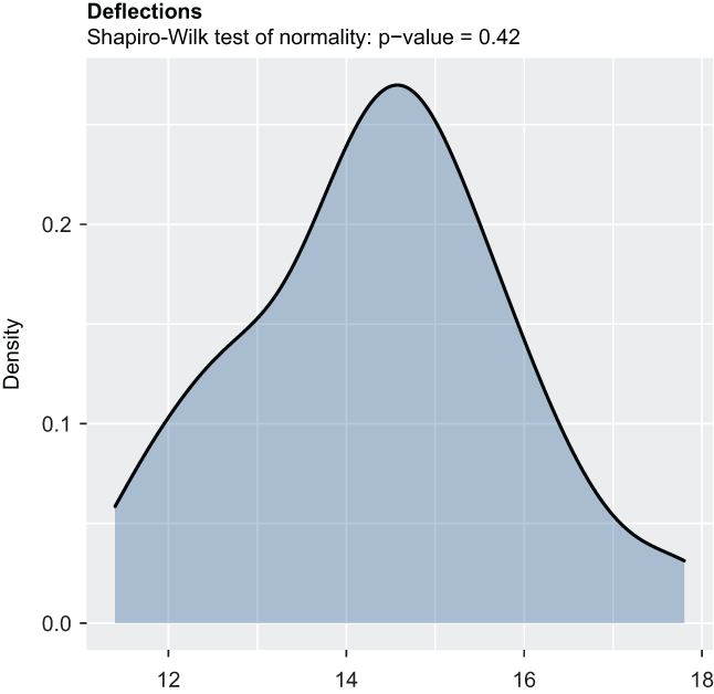
Inspect the density curve for deflections alongside its Shapiro-Wilk result to connect visual shape with a formal normality check. section 5.5.1
par(mfrow = c(2, 2))
plot(fit1)
Run base R model diagnostics to examine residual normality through the Residuals vs. Fitted and Normal QQ plots. section 5.7.5