A normal, or Gaussian, distribution is a continuous probability model whose bell-shaped density is determined by location and scale. In one dimension, μ controls the center and σ controls spread; the standard normal is N(0,1). Its multivariate form uses a mean vector μ and covariance matrix Σ. section 11.1.1 section 2.5
The distribution functions as a reusable probabilistic component:
- Model several populations with a Gaussian mixture, weighting K component distributions by positive proportions πk that sum to one. section 2.1
- Represent each sensor’s normal behavior with a Gaussian likelihood p(xi|μi,σi), then use reduced log likelihood as an anomaly signal. section 11.1.1
- Generate multivariate samples by conditioning on subsets of variables; Gibbs sampling repeatedly draws from the resulting conditional Gaussian distributions. section 2.5
For a multivariate Gaussian, partition x into xA and xB and partition μ and Σ accordingly. The conditional distribution p(xA|xB) has parameters derived from the corresponding covariance blocks, allowing one subset to be sampled while the other is fixed. If Σ = LLᵀ, samples can also be constructed as y = Lx + μ with x ~ N(0,I). section 2.8 section 2.5
Iris populations
An iris pairplot displays pairwise feature relationships and suggests modeling the three flower types as a mixture of three Gaussian distributions. Fitting the mixture requires means, covariances, and mixture proportions; expectation-maximization is deferred for parameter estimation. section 2.1
Time-series anomaly detection
An LSTM-VAE learns Gaussian output parameters for each sensor from nonanomalous data. When an input’s log likelihood drops, thresholding that decrease signals an anomaly; the latent embedding is regularized toward N(0,1). section 11.1.1
Figure 2.1 Iris pairplot: pairwise scatterplots color coded by iris species
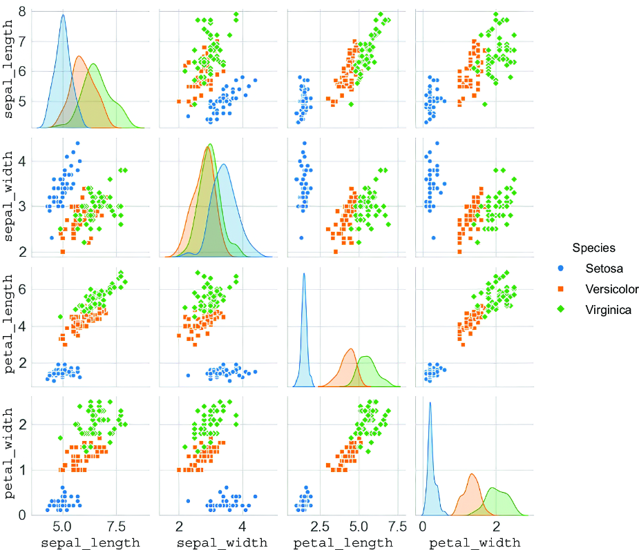
Inspect pairwise feature scatterplots and diagonal distributions to see how Gaussian components can represent iris populations. section 2.1