A normal, or Gaussian, distribution is a continuous probability distribution with a symmetric, bell-shaped density. Its shape is determined by the mean and variance: the mean locates the center, while the variance controls spread. Normality is useful as a compact description of numeric data, but statistical outlier methods often assume it only approximately. section 2.0
For multiple features, a multivariate Gaussian describes a data center and covariance matrix rather than separate means and standard deviations alone. The covariance matrix records each feature's variance and pairwise covariance, capturing elliptical shape, unequal spread, and correlations. section 5.5
Normal-distribution models support several practical interpretations:
- Use a univariate Gaussian assumption to find unusually small or large values in a numeric column. section 2.0
- Use a multivariate Gaussian to judge points relative to an elliptical data shape; covariance-aware distances can distinguish equally distant points more meaningfully than Euclidean distance. section 5.5
- Use several multivariate Gaussians when the data contains clusters generated by different processes; points far from every cluster are less probable. section 5.6
Clustered synthetic data
A Gaussian mixture model represents synthetic data with three clusters using three multivariate Gaussians, then identifies points that are unlikely under the fitted mixture. The accompanying implementation uses scikit-learn's GaussianMixture estimator. section 5.6
Figure 5.8 Data with three clusters, each captured by a multivariate Gaussian. Each location in the space has a probability, which can be estimated by the sum of the probabilities of it being generated by any one of the Gaussians, weighted by the size of each Gaussian.
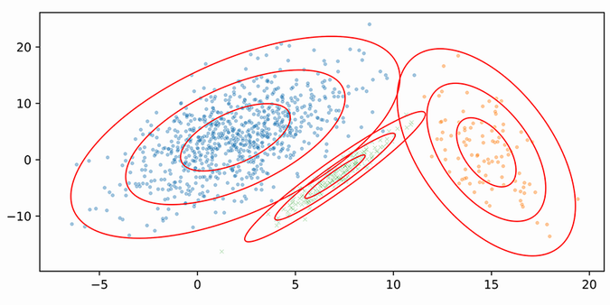
Visualizes how multiple multivariate Gaussians assign probability across clustered data and combine cluster-specific densities. section 5.6