The normal distribution, also called the Gaussian distribution, describes how continuous-valued quantities spread around a typical value. Its familiar bell-shaped curve makes it a natural model for continuous targets and regression residuals. section 7.1.2
Linear regression assumes that prediction errors follow a normal distribution. Operationally, it chooses a linear model whose residuals fit this continuous distribution rather than treating every target as a count. section 7.1.2
Use the distributional assumption to distinguish related regression settings:
- Choose a normal-error model for continuous-valued labels such as noisy measurements. section 7.1.2
- Use squared error when directly corresponding to a Gaussian residual assumption; it penalizes large errors strongly and is sensitive to outliers. section 7.3.1
- Do not use the normal model automatically for count labels: counts are discrete and often follow a Poisson distribution instead. section 7.1.2
Continuous versus count predictions
A linear regression model can represent a continuous target through normally distributed residuals. The same approach is unsuitable for visits or other counts, where predictions such as 2.41 or −4.7 are problematic and the target distribution differs. section 7.1.2
Figure 7.2 Linear regression (left) fits continuous-valued targets by assuming that the spread of the targets can be modeled by the continuous-valued normal distribution (right). More precisely, linear regression assumes that the predictions f(x) for an example x are distributed according to the normal distribution.
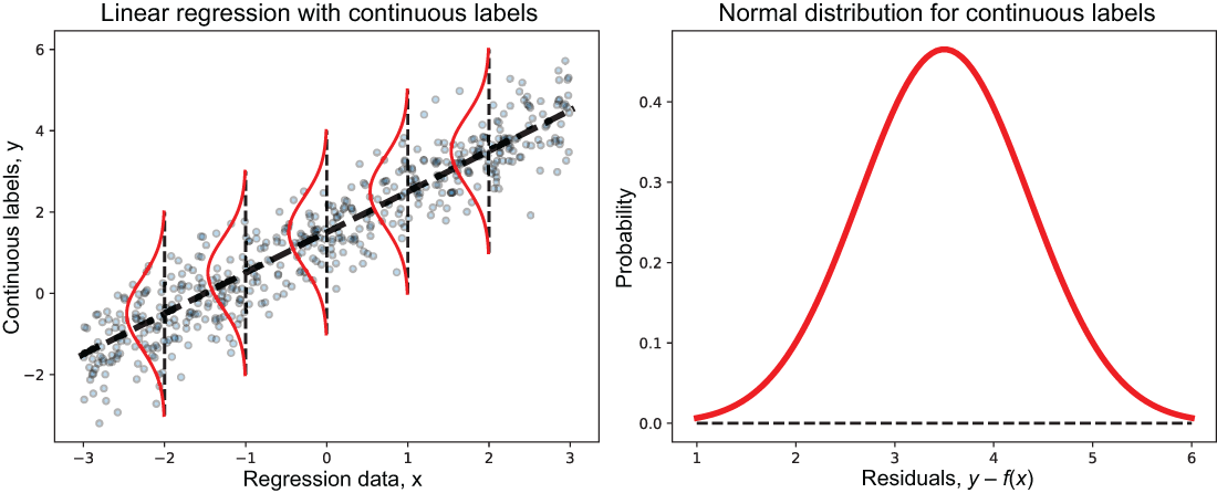
Visualize linear regression alongside normal distributions to see how the assumed spread of continuous predictions relates to the fitted line. section 7.1.2