A normal distribution, also called a Gaussian distribution or bell curve, is a continuous probability distribution shaped like a symmetric hill. Its center is the mean, where values are most common; values become less likely in either tail. The full area under the curve is always 1.0, so areas over ranges represent probabilities. section 4.1 section 4.2
Two numbers define the curve. The mean sets its horizontal location: changing it slides the curve left or right. The standard deviation sets its spread: a small standard deviation makes a narrow, tall curve with values clustered near the mean, while a large one makes a wider, shorter curve with more variability. Either way, the total area remains 1.0. section 4.2
Designing for a range of people
Adult heights provide a familiar bell-shaped example. If US women’s heights have a mean of 64 inches and a standard deviation of 2.5 inches, the center of the curve is 64 inches and most heights lie nearer that value than the extremes. A car seat adjustable from 57.5 to 70 inches would aim to accommodate a large share of people without attempting to fit every possible height. section 4.1
Figure 4.1 Normal distribution showing the height of US women
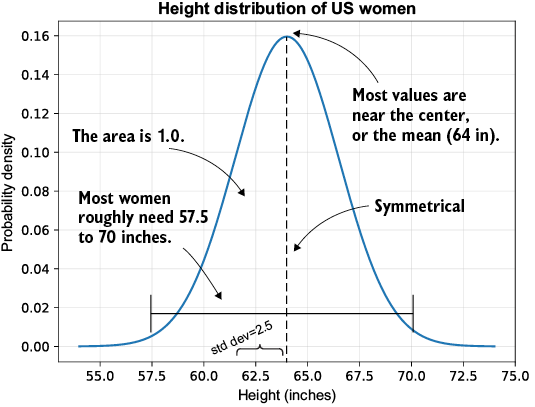
Use the height curve to see how the mean marks the center and how probability thins toward the tails. section 4.1
A bell-shaped histogram can suggest normality, but the normal curve is a probability-density model rather than a count chart. To compare a curve with observed data, scale the histogram as a density so its area, like the curve’s, equals 1. This makes the curve a useful approximation for seeing whether data cluster around a typical value with symmetric variation. section 4.3 section 4.1
Finding a reasonable coffee range
Suppose 78 baristas report how many grams of grounds make a satisfying 16-fluid-ounce pour-over. Their answers vary because tastes vary, but the mean and standard deviation summarize a typical amount and how strongly opinions differ. The sample’s mean is 27.6 grams, its median is 28.0 grams, and its sample standard deviation is 3.2 grams. Plotting a normal curve over the density-scaled responses turns “adjust to your liking” into a starting point plus a visible range to experiment with. The result still reflects who was surveyed: preferences may differ across locations. section 4.3 section 4.3
import numpy as np
from scipy.stats import norm
import matplotlib.pyplot as plt

x = np.array([27, 22, 28, 27, 26, 28, 31, 25, 25, 33, 24, 28, 28, 30,
             26, 25, 29, 28, 30, 30, 22, 28, 36, 27, 26, 31, 30, 25,
             27, 32, 25, 23, 27, 24, 28, 24, 27, 28, 30, 26, 33, 29,
             31, 29, 27, 31, 20, 23, 25, 29, 30, 24, 29, 28, 25, 25,
             30, 30, 27, 36, 26, 31, 24, 29, 34, 27, 23, 29, 27, 19,
             28, 30, 26, 29, 27, 30, 29, 28])  #1

mu, sigma = x.mean(), x.std()  #2

x_line = np.linspace(mu - sigma * 4, mu + sigma * 4, 1000)  #3
y = norm.pdf(x_line, mu, sigma)  #4
plt.plot(x_line, y)  #5

plt.hist(x, bins=np.arange(min(x), max(x) + 2) - 0.5, alpha=.4, color='#002d8b', density=True)  #6

plt.title("Ideal Coffee Grounds Amount for 16 oz Cup")  #7
plt.xlabel("Weight (grams)")  #8
plt.ylabel("Probability Density")  #9
plt.grid(True, alpha=0.3)  #10
plt.show()  #11
Inspect the code and overlay to connect raw responses, their mean and standard deviation, a density-scaled histogram, and the fitted normal curve. section 4.3
The normal distribution supports several next steps in statistical reasoning:
- Compute probabilities for value ranges with a cumulative distribution function (CDF). section 4.12
- Use the empirical rule to estimate how much data lies within one, two, or three standard deviations of the mean. section 4.12
- Connect sample means to population inference through the central limit theorem, including situations where the original data are not normal. section 4.0 section 4.12
- Provide a reference distribution for Z-tests; in practice, t-tests are often preferred because they capture greater uncertainty. section 6.3
Normality is useful, not an automatic verdict. A smooth-looking bell curve can help summarize data and make range-based probability statements, but conclusions depend on the data and sampling choices. Treat a fitted curve as a model to inspect, and keep possible bias—such as surveying only nearby coffee shops—in view when interpreting what “typical” means. section 4.3 section 4.0