A normal, or Gaussian, distribution models a continuous variable with a symmetric, bell-shaped probability density. Its mean μ sets the center; its standard deviation σ sets the spread. Density peaks at the mean and falls toward both tails. Examples include measurement errors, product weights, and regression residuals—but a bell shape should be checked rather than assumed. section 3.1.1 section 4.2.4
The probability density function is f(x) = exp(−(x − μ)² / (2σ²)) / (σ√(2π)). Its height at x is a density, not the probability of obtaining exactly x. Probability over an interval is the area under the curve between its endpoints. Symmetry puts half the area on each side of μ; increasing σ makes the curve wider and flatter. section 2.3.2 section 3.1.1
Figure 3.1 A 2 × 2 grid of normal distributions where each plot shares the same x-axis and y-axis scales. The mean equals 0 throughout, and the standard deviation equals 5, 10, 15, or 20. Increases in the standard deviation translate to greater dispersion from the mean, flatter distributions, and wider tails. In other words, the PDF becomes more dispersed across a larger range of values, and the distribution is broader and less peaked around the mean. The bell-like shape applies throughout, however, where the values are distributed symmetrically around the mean.
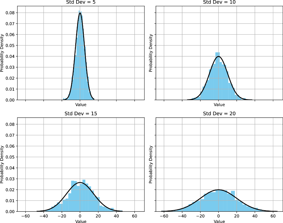
Compare curves with the same mean and standard deviations of 5, 10, 15, and 20 to see how spread changes without changing symmetry. section 3.1.1
A standard normal distribution has μ = 0 and σ = 1. Standardizing a value gives z = (x − μ) / σ: its distance from the mean in standard deviations. Use a cumulative distribution function (CDF) for the area to the left of a value; subtract two CDF values for the probability between them. In a normal distribution, approximately 68%, 95%, and 99.7% of values lie within one, two, and three standard deviations of the mean. section 3.1.1
Calculate an interval probability
With SciPy, `from scipy.stats import norm; probability = norm.cdf(1.5) - norm.cdf(1.0)` gives approximately `0.09185`: a 9.18% chance that a standard-normal value falls between 1.0 and 1.5. Use `norm.pdf(1)` instead when the question asks for density at 1; its value is approximately 0.24197, not a point probability. section 3.1.1
Applications depend on the modeling assumption. Stock-price simulations draw daily log returns from a normal distribution parameterized by historical mean and standard deviation. A project deadline calculation likewise converts a due date to a z-score before finding a completion probability. For regression, compare residuals with a normal distribution using a Q–Q plot or Jarque–Bera test; substantial departures call the assumption into question. section 9.5.1 section 13.4 section 4.2.4