A normal distribution has a bell-shaped curve, a meaningful midpoint, and roughly symmetric values on either side of the mean. Real datasets rarely fit this shape perfectly. Normality is therefore a question to investigate, not a label to assume. section 4.1.1
Normality matters when choosing an inferential test. Many parametric tests assume that the population follows a normal distribution; the observed data should be approximately normal or suitable for transformation. Inspect the distribution before using its mean or a test result to make a recommendation: datasets with similar medians can have very different shapes. section 4.2.1 section 4.1.1
A practical check is to:
- Visualize the data and look for skew, multiple peaks, and extreme outliers; consider skewness and kurtosis alongside measures of center and variability. section 4.2.1 section 4.1.1
- Try an appropriate transformation when the shape is skewed. A square-root transformation can reduce positive skew; squaring values can address negative skew. Check the resulting shape rather than assuming the transformation worked. section 4.2.1
- Choose a test with suitable assumptions if transformation fails. Uniform, extremely skewed, or multimodal data may call for a non-parametric test; categorical and discrete count data may not suit numerical transformation. section 4.2.1
Figure 4.20 The two plots on the left show the original positively and negatively skewed data, respectively. The plots on the right show the transformation of each distribution (using square root and squared values, respectively), allowing you to approximate a normal distribution.
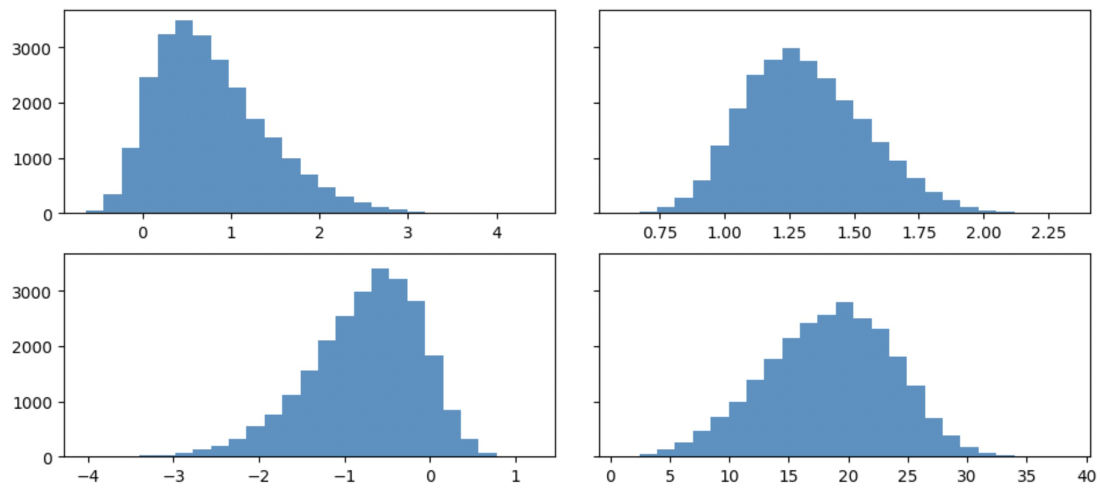
The paired histograms show positively and negatively skewed data before and after transformations intended to approximate a normal distribution. section 4.2.1
When normality changes the decision
A product analyst comparing workflow completion times across three app versions considers a between-subjects ANOVA. Each group’s distribution is bimodal, and square and square-root transformations do not bring it closer to normal. Proceeding with the ANOVA could yield unreliable recommendations about users; the analyst should consider a test with different assumptions. section 5.1
The same check arises beyond group comparisons. Linear regression includes a multivariate normality assumption about the variables in the model; a Q-Q plot is described as one way to assess it. Normality is only one assumption, so satisfying it does not by itself validate an analysis. section 4.3.2 section 4.2.1