Suppose you want to estimate how much a house’s price changes with each additional square foot. You might expect about $100, but remain unsure. A normal distribution can express both parts of that belief: a center for your estimate and a spread for your uncertainty. section 3.12
A normal distribution, also called a Gaussian distribution, is written 𝒩(μ, σ²). Its mean μ is its most likely value; its standard deviation σ describes its spread, and σ² is its variance. Its density forms a symmetric bell curve that decreases away from the mean. A larger standard deviation makes the curve wider. section 3.12
A prior with room for doubt
The prior 𝒩(100, 100²) centers the price-per-square-foot slope at $100 while allowing substantial uncertainty. About 95% of its probability lies between −$100 and $300, using the rounded interval μ ± 2σ; the more precise 95% interval is μ ± 1.96σ. The negative end matters: changing the mean or spread can make negative slopes less likely, but a normal prior cannot rule them out. section 3.12 section 5.2
Figure 3.4 The prior distribution of the slope 𝑚 in the linear regression model, which gives the highest probability to the value 100 but there’s a high level of uncertainty in this value, quantified by the large spread of the distribution.
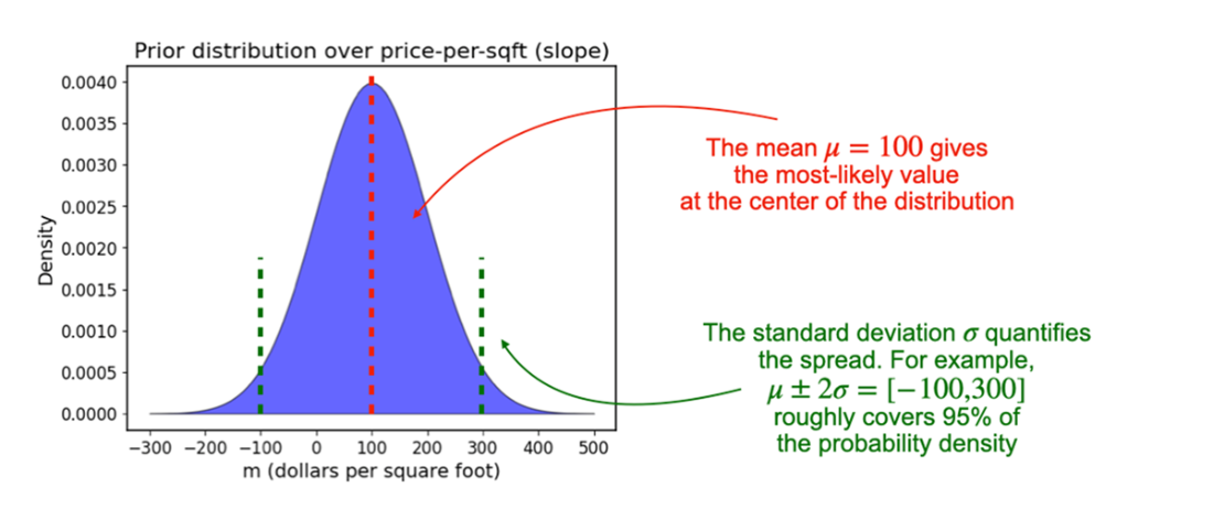
The wide bell curve makes the distinction between a most likely slope and uncertainty about that slope visible. section 3.12
Normal distributions also make a linear regression model convenient. If price is modeled as slope × area plus zero-mean normal noise, positive and negative noise are equally likely. Scaling the normal slope by area and adding normal noise still gives a normal distribution for price. With a normal likelihood, the normal prior is conjugate: the posterior for the slope is normal too. section 3.13
In variational inference, a normal distribution can instead serve as a fitted approximation to a posterior: its mean and standard deviation are adjusted to match the target. That simple shape has limits. A symmetric normal cannot exactly match an asymmetric posterior, and fitting one to a distribution with multiple peaks may concentrate it around just one peak. section 6.3 section 6.13
Comparing coaching effects
A school’s estimated average score increase can be represented as 𝒩(28, 15²): an estimated effect of 28 points with a standard error of 15. Distributions for different schools can overlap substantially, so comparing their means alone can overstate how clearly their effects differ. section 7.2