Will it rain today? The answer is unknown, but you can describe the possibilities and how likely each seems. A probability distribution does just that: it assigns probabilities to the possible values or ranges of values of a random variable. It gives a fuller picture of uncertainty than a single guess. section 1.5 section 1.0
Two possible outcomes
Let 1 mean rain and 0 mean no rain. A Bernoulli distribution uses one parameter, p: rain has probability p, and no rain has probability 1 − p. Those probabilities add to 1 because they cover both possible outcomes. section 1.5
A distribution can also describe an unknown quantity with more than two possibilities. Suppose you are estimating the proportion of people who prefer coffee over tea. You could first consider eleven values, from 0.0 to 1.0 in steps of 0.1. Assigning a probability to each value gives you a prior distribution: your view before seeing the data. Equal probabilities express no preference among those values; unequal probabilities can express a stronger belief about some of them. A continuous distribution can later account for all values between 0 and 1. section 2.9
Once data arrive, a Bayesian model updates distributions over unknown quantities. The resulting distribution retains information about which values remain plausible, rather than committing to one answer. Distributions can also connect groups: in a hierarchical model, parameters for individual groups come from a shared population distribution. section 10.0 section 7.1
Draw possible values
Sampling turns a distribution into possible values you can inspect. For a Beta(1, 1) distribution, Python’s scipy.stats provides `beta.rvs(1, 1, size=10_000, random_state=0)`. Each draw is one possible realization. A histogram of many draws approaches the distribution’s shape as the number of draws grows. section 4.1
Figure 4.1 True PDFs of Beta(1, 1) and 𝒩(100,100²) (left column) and the corresponding histograms and 10,000 samples drawn from the two probability distributions (right column). Under infinite samples, the shapes of the histograms approach the respective PDFs.
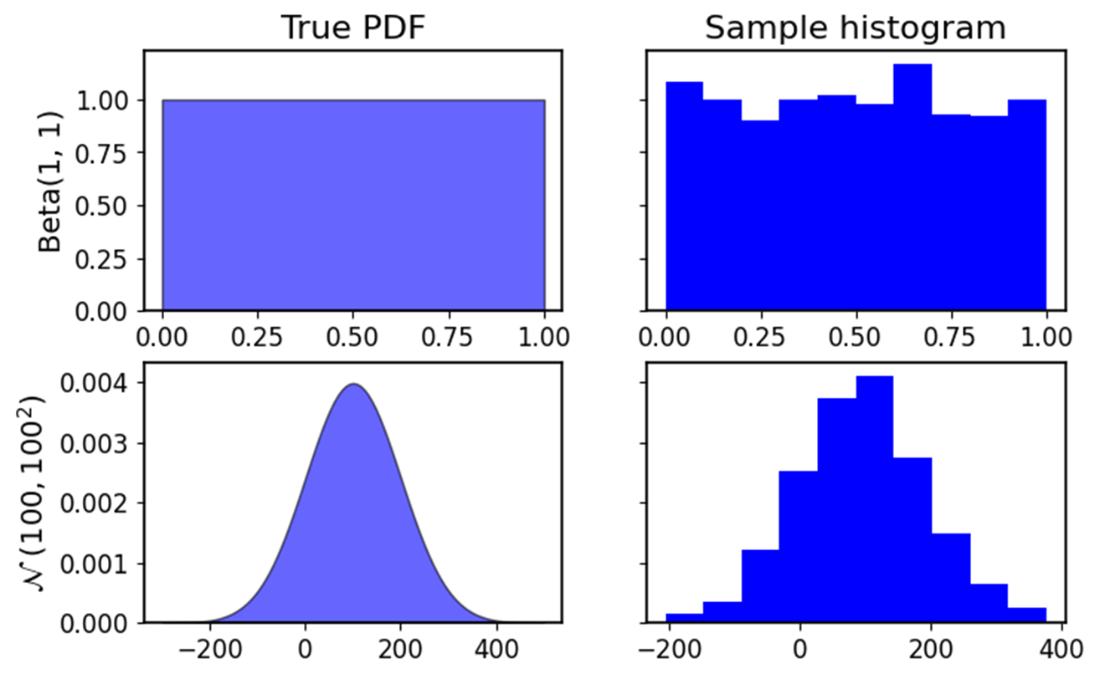
Compare each probability density curve with the histogram of 10,000 values sampled from it. The comparison makes visible how more likely regions tend to produce more samples. section 4.1